Laser writing in glass for dense, fast and efficient archival data storage – Nature

Humanity is generating data at an exponential rate, doubling approximately every 3 years (ref. ¹⁷). Much of these data hold notable personal, commercial or legal value and must be preserved for decades or centuries. Most digital archive systems rely on media that degrade within a few years^1,2,3. As a result, data must be regularly migrated to new media¹⁸, a process that is costly in time, equipment and energy.

It is, therefore, essential to find an alternative technology for the long-term preservation of digital data. Optical storage based on laser writing in glass or other durable media, termed femtosecond laser direct writing, is a promising candidate to disrupt the incumbent technologies. This is because the medium itself is thermally and chemically stable and is resistant to moisture ingress, temperature fluctuations and electromagnetic interference^19,20,21.

Here, we present Silica, a comprehensive archival digital data storage technology built on femtosecond laser direct writing in glass. Our technology guarantees data integrity (stored data are retrieved without errors), and a storage system using this technology¹⁸ guarantees high data durability (data are not lost due to failures). Silica is the first glass-based data storage that meets all the requirements of a production storage system.

Our work advances the field because we consider all main system metrics defined in section ‘Key metrics’. Our comparison with known previous work^{4,5,6,7,8,9,10,11,12,13,14,15,16,22} (Supplementary Information) shows that, to our knowledge, Silica is the first published storage technology using glass that performs across all these key storage metrics and is the first to demonstrate reliable operation across writing, reading and decoding.

Our work is based on several key innovations:

• Two efficient regimes of volume pixel (voxel) writing in glass: we use phase voxels relying on isotropic refractive index (RI) changes and birefringent voxels based on anisotropic changes (see section ‘Writing data’). We demonstrate high-quality voxels, each storing more than one bit, using a minimum number of pulses.

• High-throughput, stable writing: we demonstrate writing at high throughput using multiple beams per laser (Extended Data Fig. 4). We use a closed-loop feedback system to actively monitor and optimize the laser power, providing precise energy stability during writing and enabling predictability and reliability across different writers at scale (see section ‘Emissions-based control of voxel writing’).

• Data retention characterization: we develop a methodology to characterize the lifetime of the data stored in glass separately from the lifetime of the glass media (see section ‘Lifetime’).

• Machine learning decode: building on our previous work²³, here we apply machine-learning-based decode (see section ‘Reading and decoding data’) to account for noise and inter-voxel cross-talk.

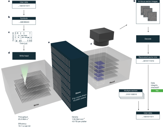
The high-level organization of Silica is shown in Fig. 1. User data is received as a stream of bits, to which additional bits are added using forward error correction (FEC) (Fig. 1a). This ensures data integrity despite stochastic errors during writing and reading. Bits are then grouped into symbols (Fig. 1b). Each symbol corresponds to a voxel and stores more than one bit. The laser energy or polarization is modulated as the beam is moved relative to the glass sample (Fig. 1c, platter). Voxels are written in two-dimensional (2D) planes and stacked into three-dimensional (3D) volumes (Fig. 1d). In each plane, voxels are organized into sectors based on the field of view (FOV) of the read system. Sectors are stacked vertically into tracks. We read using wide-field microscopy (Fig. 1f). Symbols are inferred from images using convolutional neural networks (CNNs; see section ‘Reading and decoding data’) and then decoded into user bits (Fig. 1g).

We compare Silica with other storage technologies in the Supplementary Information. a, Data are received from a user. These are prepared as a stream of bits, for example, using compression, encryption and FEC. b, The bits are encoded as symbols. One symbol corresponds to a modulator configuration. c,d, The glass sample is loaded into a write subsystem and the modulator settings are changed in time as the laser beam is moved relative to the glass. The symbols are written layer by layer, from the bottom up, to fill the full thickness of the glass. e, The data can be stored securely in the glass for more than 10,000 years. f, To read, we use an automated microscope with a camera to capture images of each 2D layer of voxels. g, Images are passed to a decoder to recover user data.

Source Data

Full size image

All steps, including writing, reading and decoding, are fully automated, supporting robust, low-effort operation. This automation allows us to characterize the stability of the technology at scale, using repeated writes and reads of billions of bits of data. We demonstrate longevity of the written data using accelerated ageing experiments. We project that the data are stable for more than 10,000 years at room temperature (Fig. 1e), demonstrating the archival potential of the medium. We demonstrate data integrity (see section ‘Silica system analysis’) by verifying that all the written data are decoded back without errors, whereas data durability is enabled by cross-track and cross-platter data redundancy¹⁸.

This whole-system approach enables a rigorous and comprehensive evaluation of an archival storage technology based on glass, establishing Silica as a future-proof archival solution for the digital age.

In this section, we introduce the innovations in femtosecond laser writing that underpin Silica. Existing works are limited in throughput and efficiency, in part because many rely on multiple laser pulses per voxel^10,24,25,26. To overcome these limitations, we developed two advanced regimes: pseudo-single-pulse writing of birefringent voxels and single-pulse writing of phase voxels. These approaches maximize energy efficiency and enable write throughput to reach the laser repetition rate. The resulting weak modifications allow us to improve density substantially beyond reported approaches because they exhibit low scattering and cross-talk and so enable data writing and reading from more than 300 layers^10,25,27 (see section ‘Reading and decoding data’).

The write subsystem shown in Fig. 2a contains a femtosecond laser source, polarization or amplitude modulators for data encoding (Fig. 2b), opto-mechanical beam scanning elements and a high-precision focusing objective with an adjustable collar for spherical aberration correction. Any component of this subsystem can introduce spatial and temporal energy fluctuations, degrading voxel quality. We compensate for spatial inhomogeneities by using the results of an offline calibration to adjust the symbol modulation (see section ‘Emissions-based control of voxel writing’). We compensate for temporal fluctuations (Fig. 2c) using a closed-loop control system that dynamically adjusts pulse energy to maintain a target level of plasma emissions²⁸ (see section ‘Emissions-based control of voxel writing’).

a,b, Setup (a) and modulation methods (b) for birefringent and phase voxels. c, Emissions monitoring to enable consistent data writing. d, Schematic of pseudo-single-pulse writing of birefringent voxels and scanning electron microscopy (SEM) top-view image of elongated nanovoids in fused silica, e,f, Schematics of single beam (e) and multibeam (f) single-pulse writing of phase voxels. In e, the SEM and phase-contrast microscopy (PCM) images show top-view and side-view profiles, respectively, of the different phase voxel symbols written in borosilicate glass. EOM, electro-optic modulator; AOM, acousto-optic modulator; RF, radiofrequency. a.u., arbitrary units. Scale bars, 200 nm (d, top); 2 μm (d, bottom; e, middle and bottom; f, bottom); 500 nm (e, top).

Source Data

Full size image

Pseudo-single-pulse writing of birefringent voxels

Birefringent voxels are composed of optically anisotropic sub-diffraction modifications, the in-plane orientation of which is determined by the polarization of the writing pulse. Varying this orientation encodes different data symbols^5,6,7,9,10, which we read using polarization-resolved imaging (see section ‘Reading and decoding data’). Three types of birefringent voxels have been observed in fused silica glass. Our preferred type is elongated nanovoids¹⁰, which we discuss in detail below. Alternatively, we can use either (1) nanogratings^5,6,7,29 or (2) ensembles of elongated nanopores⁹. The first option is not desirable because nanogratings exhibit high scattering and induced residual stress. We explored the second option with a continuous writing regime (Extended Data Fig. 1), but here a large writing energy is required and throughput is limited due to thermal accumulation.

Our new pseudo-single-pulse regime shows the formation of elongated nanovoids with just two pulses, improving on previous work¹¹. We split each pulse into two: one that forms a void (seed pulse) and the other that elongates a previously formed void (data pulse). These are separated along the beam scanning direction, typically by two to three times the voxel pitch. We split the pulses using a tunable beam splitter (see section ‘Writing birefringent voxels by pseudo-single-pulse regime’). In this way, a single laser pulse simultaneously initiates the formation of a new seed structure and converts an existing seed structure into a data voxel, so voxels are written at the laser repetition rate of 10 MHz (Extended Data Fig. 2). We modulate the pulses before splitting because we discovered that the voxel azimuth is determined only by the polarization of the data pulse. We write with elliptical polarization to reduce modulator driving voltage²⁴.

Phase voxels by single-pulse writing

Phase voxels are femtosecond-laser-induced isotropic modifications with locally altered RI and minimal optical scattering. The pulse energy is modulated to encode the symbol. These modifications have been observed in various types of transparent materials^21,30,31,32. In our work, we write in borosilicate glass (Fig. 2e–f). Each voxel is written with a single pulse, so voxels are written at the laser repetition rate of 10 MHz. We modulate the beam energy using an acousto-optic modulator (AOM; see section ‘Writing phase voxels’). Different symbols correspond to distinct RI changes that can be read using Zernike phase-contrast microscopy³³ (Extended Data Fig. 3; see section ‘Phase read’).

Furthermore, we demonstrate a throughput of 65.9 Mbit s⁻¹ by splitting the laser into 4 independently modulated beams. We scan all beams with the same scanner and objective (Fig. 2f and Extended Data Fig. 4). The written, read and decoded results show that throughput can be scaled in this way without damaging the media.

After writing, we perform reading and decoding to recover the original data. We read using wide-field transmission optical microscopy, which allows us to read the voxels in parallel (see section ‘Read hardware’). A detection numerical aperture (NA) of 0.6 is used; lower NA values do not sufficiently resolve signals from adjacent voxels, whereas higher NA values introduce more significant spherical aberration with depth^34,35,36. We read a track of data by translating the glass in z while adjusting the spherical aberration correction collar of the objective, and then move in xy to the next track. We use an autofocus algorithm to acquire images of each sector at the correct focal position.

For birefringent voxels, the in-focus images corresponding to a single sector are acquired from a single z plane at different polarization states (Fig. 3a). For phase voxels, the phase-contrast pupil-plane filters elongate the point-spread function in the axial direction. To mitigate this effect, we acquire images from multiple z positions to decode each sector (Fig. 3b; see sections ‘Phase read’ and ‘Machine learning model’).

a, Schematic of birefringent voxel readout using polarization-resolved microscopy. b, Schematic of phase voxels readout using phase-contrast microscopy. c, Decode pipeline showing images being decoded into recovered sectors. d, LDPC curves showing the trade-off between code rate (horizontal axis) and quality factor (vertical axis) for birefringent and phase voxels, written under state-of-the-art conditions detailed in section ‘Silica system analysis’. e, Example heatmap of code rates required to recover the original data encoded in phase voxels across layers (vertical axis) and tracks (horizontal axis). The data indicate the code rate is mostly dependent on depth in the glass rather than xy position. OL, objective lens.

Source Data

Full size image

After acquisition, images are passed to our decode pipeline, consisting of four steps: pre-processing, symbol inference, symbol-to-bit mapping and error correction (Fig. 3c; see section ‘Machine learning model’). For symbol inference, we use a CNN trained on experimental data (see section ‘Machine learning model’). This outputs symbol probabilities for each voxel. For debugging and working with small quantities of data, for example, in calibration experiments, we can decode without a CNN (Supplementary Information).

The symbol probabilities are converted to bit probabilities by a predetermined mapping (see section ‘Extending binary Gray codes’). A low-density parity-check (LDPC) code³⁷ is used to correct errors in each sector. To evaluate how hardware changes affect the quality factor and therefore all key metrics (see section ‘Key metrics’), we developed a method for selecting the LDPC code rate (useful bits divided by total bits) to trade-off redundancy within sectors (to correct bit errors) and across sectors (to recover from sector loss) (see section ‘Redundancy optimization and error correction’). The best code rate achieves the highest possible quality factor and corresponds to the peak of the curve in Fig. 3d. The quality factor gives a more accurate measure of decoding performance than raw bit error rate (BER) or symbol error rate (SER) because it indicates how much redundancy is needed to faithfully recover all the user data.

Figure 3e shows a heatmap of the maximum code rate across depth and tracks. The results of this plot have two important implications for estimating the voxel quality of a whole platter: first, as the variation between tracks is not significant, we can obtain a reasonable estimate by reading and decoding a subset of the written tracks; second, as the variation within each track is significant, we must read every sector in each track in the subset. The plot also shows that layers 200–250 see a slightly worse code rate than others. We know this is a read-side effect because when reading the glass upside down, this code rate trend is reversed. We use billions of voxels in each experiment: these come from more than 200 tracks, each containing more than 250 sectors, and each sector consists of more than 20,000 voxels.

Having described how we write, read and decode data, we now present a full system analysis of the Silica platform. In Extended Data Table 1, we summarize the key properties of both the birefringent and phase voxel regimes and include results from the multibeam writing system for phase voxels.

Using birefringent voxels, in fused silica glass, we achieve 1.59 Gbit mm⁻³ data density (usable capacity of 4.84 TB per platter, 0.500 μm × 0.485 μm voxel pitch and 6 μm layer spacing, 301 layers, 8 azimuth levels at 0.85 quality factor), a write throughput of 25.6 Mbit s⁻¹, and a write efficiency of 10.1 nJ per bit.

Using phase voxels, in borosilicate glass we achieve 0.678 Gbit mm⁻³ data density (usable capacity 2.02 TB per platter, 0.5 μm × 0.7 μm voxel pitch, 7 μm layer spacing, and 258 layers, 4 energy levels at 0.92 quality factor), a write throughput of 18.4 Mbit s⁻¹, and a write efficiency of 8.85 nJ per bit. Furthermore, our multibeam system achieves a throughput of 65.9 Mbit s⁻¹ through parallel writing with four beams without inducing thermal damage. Thermal simulations indicate that writing with 16 or more beams should be possible (Extended Data Fig. 5).

Although the metrics achieved with birefringent voxels are higher, phase voxels present other advantages (see section ‘Future scaling and conclusion’).

Optimizing parameters at each pitch

To choose the best operating parameters for phase Silica, we consider data density, write efficiency, and write throughput per laser beam. All metrics are dependent on voxel quality (see section ‘Key metrics’). Density is proportional to the number of voxels per unit volume, write efficiency to laser pulse energy, and write throughput to laser repetition rate and number of beams. Therefore, given a fixed laser repetition rate and number of beams, we account for all key metrics by jointly optimizing density and voxel quality. The former is desirable because it reduces both per-bit cost of the media and mechanical overheads, whereas the latter affects all the metrics, making it key to overall system performance. This joint optimization is a trade-off because voxel quality is low at the highest density points. Figure 4a shows an example of voxel pitch optimization (x, y and z spacing). This plot shows just a few key points selected from hundreds of pieces of glass at different pitches. The dashed grey line shows the Pareto front: points on the line offer efficient trade-offs, whereas points below and to the left of the line are dominated by others and may be ignored. The point 0.5 μm × 0.7 μm × 7 μm delivers 2.02 TB per platter of usable capacity, at a voxel quality of 1.84 bits (for phase voxels).

a, Plot of density and voxel quality for different xyz phase voxel pitches (in μm). b, Example response of a phase voxel channel shown as predicted modulation compared with input modulation. The colour scale shows the model’s estimate of the likelihood of each output value given the input. c, Finding the best symbol count and write target emission for a given voxel pitch. d, Quality factor and density for repeated reads and writes showing the robustness of Silica results. Different colours correspond to different write repetitions of the same data. e, Arrhenius plot of decay time against temperature (inset actual, outer extrapolated) suggesting a voxel lifetime that exceeds 10,000 years at 290 ^°C. a.u., arbitrary units.

Source Data

Full size image

The optimal operating parameters for Silica are expected to vary with glass composition²¹ because the intrinsic material properties influence voxel formation behaviour. This work should be repeated in order to evaluate alternative glasses.

For each voxel pitch experiment, we optimize across the photo-induced emission used for closed-loop feedback control (see section ‘Emissions-based control of voxel writing’), the number of bits per voxel, and the energy modulation for each symbol. We optimize at a given pitch by sweeping only the emission parameter on a single glass sample. We need an experimental method to optimize the number of symbols and the energy modulation per symbol because the apparent voxel intensity in the image is a nonlinear function of the energy modulation, and the system exhibits symbol-dependent noise (see section ‘Symbol selection optimization’). Figure 4b shows a prediction of the energy modulation ((widehat{Y}), vertical axis) as a function of the known energy modulation (Y, horizontal axis). The energy modulations are normalized relative to the energy corresponding to the emission used in the experiment. At low Y, no voxels are formed, so (widehat{Y}) is flat here. As Y increases, there is a region of unpredictable and unusable modification. At higher Y is the region of predictable and useful modulation.

Figure 4c shows, for just one example pitch, the write efficiency for each set of optimized symbols on the vertical axis (lower values preferred) against number of symbols on the horizontal axis, and the swept emissions value in colour. With too few symbols, the channel is underused; with too many symbols, more redundancy is needed, which results in low code rates and, therefore, poor write efficiency.

Experimental repeatability

To evaluate the robustness of the Silica system, we wrote the same data into three pieces of glass and read each one 11 or more times for a total of 37 reads (over several months) (Fig. 4d). For each read, we decoded the data and found the best operating point on the LDPC curve to get a quality factor and corresponding data density. We plot each read as a dot, coloured by the corresponding written glass sample. We overlay a box-and-whisker plot for each glass sample giving the median (red line), interquartile range (IQR, box), and minimum and maximum (whiskers) of the quality factor. The data show that the variability across reads is small: averaged across the three glass samples, the quality factor IQR is 0.00230, leading to an IQR of 1.69 Mbit mm⁻³ in density (that is, 0.25% of the median density). The quoted headline figure of 0.678 Gbit mm⁻³ corresponds to the best read (that is, maximum density) of glass sample B in Fig. 4d.

Lifetime

To assess the thermal stability of phase voxels, we perform accelerated ageing experiments based on the Arrhenius law, using visible light diffraction measurements to track the decay of written structures (see section ‘Lifetime conditions’). Figure 4e shows an Arrhenius plot relating the characteristic 1/e decay time τ to temperature T. Extrapolation from the measurement points at elevated temperatures suggests exceptional long-term stability, indicating a modification lifetime that exceeds 10,000 years at 290 °C and therefore even longer at room temperature. This lifetime reflects the thermal stability of phase voxels under isolated conditions and does not account for external influences, such as mechanical stress or chemical corrosion, which are beyond the scope of this study.

A key system choice for a future Silica system is whether to use birefringent or phase voxels. We have shown that birefringent voxels achieve higher key metrics than phase voxels. However, efficient formation of birefringent voxels can be achieved only in high-purity silica glasses, whereas phase voxels can be written in potentially any durable transparent media, for example, borosilicate glass as demonstrated here. For phase voxels, the writing and reading hardware are simpler, requiring only one modulator per beamline and only one camera per reader, respectively. Both regimes can match the maximum laser repetition rate of 10 MHz or higher.

In future, Silica can take advantage of continued advancements in write, read, decode hardware, machine learning models and the commoditization of key components. Progress in any of the underlying technologies, but especially femtosecond lasers, will improve the technology.

Increasing the writing NA from 0.6 to 0.85 could halve the write energy and reduce the voxel volume by four times, assuming that write energy, voxels per unit lateral area and layers per unit axial length are proportional to NA². Alternative glass compositions could allow higher voxel quality and write efficiency, for example, if they have a lower threshold for energy modification. Write throughput can also be scaled using off-the-shelf femtosecond lasers operating at 50 MHz or higher, combined with spatial multiplexing across hundreds of beams.

Read throughput is dependent mostly on camera specifications and large FOV high-resolution optics. The absolute read throughput was not considered in this paper as it is not a significant cost component of the system¹⁸.

A full archival system in the cloud would require consideration of many other computer system design aspects¹⁸. There, glass handling between write and read subsystems would be automated by a robotic glass library^18,38.

In conclusion, we have demonstrated Silica, an optical archival storage system that uses femtosecond laser writing in glass. We show two new regimes for writing data in glass based on birefringent voxels and phase voxels. Both regimes make best use of the laser by minimizing the number of pulses required to write each voxel, achieving high write throughput and energy efficiency as well as high density. The fully automated nature of our write hardware, read hardware and decode pipeline allows us to show the robustness of our key results across many billions of voxels. We demonstrate that Silica is a viable storage system by fully recovering user data using FEC, and show through accelerated ageing experiments that our modifications last more than 10,000 years at room temperature. In short, our results demonstrate that Silica could become the archival storage solution for the digital age.

Key metrics

We evaluate the Silica storage system against the following metrics:

• Voxel quality, Q = B/n_V, is an average (bit per voxel) calculated from the number of user bits, B, stored in a large number of voxels, n_V. Q < Q_w, where Q_w is total number of bits per voxel, because redundant bits are added to correct for errors. We define q = Q/Q_w as the quality factor (see section ‘Redundancy optimization and error correction’). All other metrics except lifetime are dependent on Q.

• Data density, ρ = Q/V is the voxel quality that can be stored in a volume V of glass (Gbit mm⁻³), where V is computed as the product of the x pitch, y pitch and the effective z pitch (that is, the total 2 mm thickness of glass divided by the number of layers written).

• Usable capacity is the total number of user bits that can be stored in a single glass platter 120 mm square and 2 mm thick, reduced by a factor of 0.747 to account for engineering overheads, measured in TB per platter.

• Write throughput, θ = fN_LQ, where f is the laser repetition rate and N_L is the number of beam lines, is the speed at which data can be written to the glass, measured in bit s⁻¹. It is defined as a peak throughput.

• Write efficiency, η = E/Q measures the energy consumed to write each user bit (nJ per bit). E is measured after the objective. A lower η represents better write efficiency and so is preferred as it allows more bits to be written in parallel for the same laser pulse energy.

• Lifetime is an experimental estimate of the lifetime of the data stored in the glass (see section ‘Lifetime’).

Write

Figure 2a shows the key building components of the data writing system. The source is an amplified femtosecond laser (Amplitude Systems, Satsuma HP3 with harmonic generation, 516 nm central wavelength (second harmonic), and tunable pulse duration from 300 fs to 1,000 fs). We measured the pulse duration before the objective lens using a Gaussian fit of the autocorrelator signal (APE, Carpe). The output laser pulse train at 10 MHz passes through a tunable attenuator, quartz half-wave plate on a motorized rotary stage and Glan linear polarizer.

After the attenuator, the optical configuration depends on the type of voxel being written. Birefringent voxel writing requires polarization modulation and beam splitting, the latter to generate seed and data pulses. Phase voxel writing requires only amplitude modulation.

The modulated laser pulses are collimated and incident on a self-air-bearing polygon scanner (Novanta, SA24) with 24 facets spinning at 10,000–50,000 rpm. The scanned laser pulses are directed through a custom-made f-theta scan lens (focal length = 63 mm) followed by a relay lens. This optical arrangement ensures that the pulses consistently enter the objective pupil, regardless of the scan angle.

The objective (Olympus, LUCPLFLN40X) focuses the scanned laser pulses inside the glass platter (2 mm thickness), which is mounted on an xy translation stage (PI, V-551.7D and 551.4D). The translation stage moves at a constant velocity along the x-axis, whereas the pulses are scanned along the y-axis so that we write a plane of voxels at constant depth. We choose the velocity of the stage and the spinning rate of the polygon so that the laser pulses are focused at the intended pitch, for example, about 3.57 mm s⁻¹ and 17,000 rpm for an intended pitch of 0.5 μm × 0.7 μm in glass. The relation between the velocity, the spinning rate and the pitch is given by the repetition rate of the laser pulses, the magnification from the polygon facet to the objective lens, the number of polygon facets per rotation and the focal length of the objective lens (Supplementary Information).

The writing depth in the glass is changed by translating the objective lens in z while using an in-house-designed, motorized actuator to adjust the spherical aberration correction collar of the objective. The CMOS (complementary metal-oxide semiconductor) sensor (FLIR, GS3-U3-41C6M) captures the photoemission images during writing through the same objective as the write laser beam. The images are used for the closed-loop control to stabilize the voxel writing (for more details, see section ‘Emissions-based control of voxel writing’).

We stabilized the rotational speed of the polygon using a photodiode that detects a fixed continuous wave laser beam (632 nm, Thorlabs, PL202) reflected off the polygon facets. The beam, on a separate path from the writing laser, sweeps across the photodiode once per facet, generating 24 spikes per revolution. These spikes provide feedback to control the polygon motor speed. To account for the difference in polygon facet reflectivity, we measured the photoemission intensity from a line of voxels written with each polygon facet and use this as a calibration signal to feed in to the AOM (for more details, see section ‘Emissions-based control of voxel writing’).

The energy per voxel (EPV) is determined by measuring the average laser power after the objective lens with a thermal power meter (Thorlabs, PM101A). EPV is measured only for the strongest symbol; therefore, it represents the energy requirement before amplitude modulation. This value is used to estimate write efficiency, excluding losses from optical bench components.

Birefringent voxels are written in fused silica glass (Heraeus, Spectrosil 2000). Phase voxels are written in borosilicate glass (Schott, BOROFLOAT 33).

Writing birefringent voxels by pseudo-single-pulse regime

Between the tunable attenuator and polygon scanner, there are two key modules required for writing birefringent voxels with the pseudo-single-pulse regime: a tunable beam splitter and a polarization modulator.

Tunable beam splitter

The attenuated laser beam is split into two beams (seed and data) with either an acousto-optic deflector (AOD) (G&H, AODF 4140) or polarization grating (PG) beam splitter. The AOD splits the laser beam at an arbitrary angle and power ratio by tuning the radiofrequency signal. We typically use an energy ratio of 100:60–70 for the seed:data pulses. The PG beam splitter, consisting of a pair of PGs, splits a laser beam into two, the angle and power ratio of which can be tuned by changing the relative angle of the PGs and the polarization of the input beam (Supplementary Information). We tune the split angle between the seed and data beams to make the distance between the seed and data pulses inside the glass equal to a multiple of the voxel pitch, so that the data pulse hits the seed structure created by the seed pulse. Our best density was achieved using a spacing between seed and data beams of three voxel pitches at a voxel pitch of 0.485 μm.

Polarization modulator

After splitting, the two beams pass through a relay lens and are directed into two sequentially arranged Pockels cells (ADP, Leysop, EM200A-HHT-AR515), with a relative crystal orientation of 45°. The two Pockels cells modulate the polarization of each pair of pulses (both seed and data beams simultaneously). We write with elliptical polarization (ellipticity = 0.5) to reduce the Pockels driving voltages. We use our own custom-made high-voltage modulators to modulate the Pockels cells (200 V peak-to-peak amplitude with 10 MHz bandwidth). The polarization is unintentionally modified by some of the optical components after the Pockels cells. We compensate for this modification using a pair of wave plates after the Pockels cells, tuned so that the polarization at the objective pupil is circular when both modulators are set to 0 V.

Writing phase voxels

Between the tunable attenuator and the polygon scanner, the beam passes through a module responsible for amplitude modulation. After passing through a tunable attenuator, the beam is reduced to a diameter of 0.5 mm or less and directed through a quartz AOM (G&H, I-M110-2C10B6-3-GH26) for beam deflection and amplitude modulation. This spot size ensures the modulation rise and fall time is less than 100 ns. The AOM is modulated with a radiofrequency signal that is frequency-locked to the laser. The radiofrequency signal encodes the data and modulates the diffraction efficiency of each pulse. We use the first diffracted order for writing.

For multibeam writing, we split a laser beam from the same source (Coherent, Monaco 517-20-20, 10 MHz repetition rate and 517 nm central wavelength, 310 fs pulse duration) into four beams, each of which is modulated with its own AOM and made to propagate closely together by a beam position controller with edge mirrors. The beams are scanned with the same polygon facet and incident on a single objective lens at slightly different angles perpendicular to the scanning direction. The objective lens focuses the four pulses at different locations inside the glass. More detail on the multibeam setup is provided in Extended Data Fig. 4, and the thermal simulation methodology is described in Supplementary Information.

Emissions-based control of voxel writing

White light emission arises during writing from the generation of a dense and hot plasma during voxel formation²⁸. The write objective is used to collect this emission in a back-reflection configuration. The emission is transmitted through a dielectric mirror (the same mirror that deflects the writing beam in the forward pass) and imaged using a tube lens and relay optics onto a camera sensor (2,048 × 2,048 pixels, 8-bit FLIR, Grasshopper3, GS3-U3-41C6M-C). The scanning line (length up to 300 μm) is magnified on the camera sensor to ensure at least 3 pixels per 0.5 μm inside the glass. A notch wavelength filter is installed to remove scattered laser light. The emission profile along the scan line is obtained by first integrating the pixel intensities vertically and then binning horizontally to obtain a 128-point signal. The sensor is rotated about the optical axis to avoid interference effects between the sensor rows and the emissions line.

The emission-based control has two aspects: offline flattening and closed-loop control. Offline flattening compensates static differences at different points in the scanning space, for example, caused by reflectivity of the polygon facets. Closed-loop control compensates dynamic differences during the writing process, for example, temperature fluctuation, by controlling the laser power with the AOM to reach a specified emission target.

The offline calibration of the non-linearity in the electronics and AOM, the spatial variation in the polygon and scan optics, and the depth-dependent variation in the objective are done by a combined procedure. The laser is set to a fixed energy just below the damage threshold, and the AOM modulation is swept from the modification threshold to maximum, forming voxels at multiple depths in the glass. Hence, for every element in depths × facets × scan angles, we have a mapping from modulation to emission. We invert this mapping using quadratic fits to obtain the dynamic modulation required to achieve a flat target emission. This is stored and then superimposed with the symbol modulation during subsequent data writing.

In closed-loop control, a target emission value is defined for each sample. This value is relative and may vary between experiments and writing systems. Writing proceeds along the x-axis in sequences called supersectors. Each supersector begins with a few pad sectors, written using only the highest amplitude symbols. These pad sectors allow the writer to measure the initial emission profile and adjust the laser power using the AOM. After each supersector is written, the writer uses the pad sectors to iteratively tune the AOM modulation until the emission aligns with the target value. This tuning process is repeated as needed. Closed-loop control resets at the start of each layer, and the camera shutter time is configured to integrate over at least one full polygon revolution to ensure consistent emission measurement.

After writing the final supersector of each layer, we measure the EPV to track the absolute energy metric, as described in the section ‘Write’. For more details on emissions-based control, see Extended Data Fig. 6.

Write conditions of data samples

Phase voxels

The write conditions for data samples are as follows: about 16–19 nJ at 1.9–0.1 mm glass depth, respectively, measured after objective; 400 fs pulse duration before the objective; 0.5 μm × 0.7 μm voxel pitch, 7 μm layer spacing and 258 layers; borosilicate glass (BOROFLOAT 33, Schott); phase voxels regime (isotropic RI change); 516 nm wavelength; NA 0.6 (40×) focusing objective (Olympus, LUCPLFLN40XRC); single-pulse per voxel at 10 MHz laser repetition rate (Satsuma, Amplitude); four levels of amplitude modulation; synchronized polygon scanning (Novanta, SA24) and XYZ (PI) media and objective translation.

Phase voxels for symbol count and modulation optimization

The conditions for symbol count and modulation optimization are as follows: about 16 nJ–20 nJ to about 19 nJ–23 nJ at 1.9–0.1 mm glass depth, respectively, measured after objective; 400 fs pulse duration before the objective; 0.5 μm × 0.7 μm voxel pitch, 7 μm layer spacing and 258 layers; borosilicate glass (BOROFLOAT 33, Schott); phase voxels regime (isotropic RI change); 516 nm wavelength; NA 0.6 (40×) focusing objective (Olympus, LUCPLFLN40XRC); single-pulse per voxel at 10 MHz laser repetition rate (Satsuma, Amplitude); 31 levels of amplitude modulation; synchronized polygon scanning (Novanta, SA24) and XYZ (PI) media and objective translation.

Phase voxels for multibeam analysis

The conditions for multibeam analysis are as follows: about 17–19 nJ at 1.9–0.1 mm glass depth, respectively, measured after objective; 310 fs pulse duration after the objective; 0.5 μm × 0.7 μm voxel pitch, 7 μm layer spacing, and 258 layers; borosilicate glass (BOROFLOAT 33, Schott); phase voxels regime (isotropic RI change); 517 nm wavelength; NA 0.6 (40x) focusing objective (Olympus, LUCPLFLN40XRC); single-pulse per voxel at 10 MHz laser repetition rate (Monaco 517-20-20, Coherent); four levels of amplitude modulation; synchronized polygon scanning (Novanta, SA24) and XYZ (PI) media and objective translation.

Birefringent voxels written by pseudo-single-pulse regime

The write conditions for birefringent voxels written by pseudo-single-pulse regime are as follows: about 22–26 nJ at 1.9–0.1 mm glass depth, respectively, measured after objective; 300 fs pulse duration before the objective; 0.500 μm × 0.485 μm voxel pitch, 6 μm layer spacing and 301 layers; fused silica glass (Spectrosil 2000, Heraeus); elongated single nanovoid voxels regime (birefringent modification); 516 nm wavelength; NA 0.6 (40×) focusing objective (Olympus, LUCPLFLN40XRC); pseudo-single-pulse per voxel at 10 MHz laser repetition rate (Satsuma, Amplitude); eight levels of polarization modulation; synchronized polygon scanning (Novanta, SA24) and XYZ (PI) media and objective translation.

Read hardware

For both birefringent and phase voxels, we read using a wide-field microscope with an sCMOS (scientific CMOS) camera (Hamamatsu ORCA Flash4 v.3.0, 2,048 × 2,048 pixels, 6.5 μm pixel size) and LED illumination. The glass is mounted in a custom-made sample holder that is mounted on a mechanical xyz stage.

The illumination, mechanical motion of the sample and the camera are all controlled by custom software developed in-house.

At write time, several fiducial markers are written into the glass at predetermined locations, and the data location is known relative to these markers. The read subsystem finds these fiducial markers and uses them to calibrate the glass position so that any track or sector can be located automatically.

To record all images for sectors in a track, we first need to find the in-focus positions of each sector. To do this, the sample is first continuously moved in the z-direction with the camera running at a fixed frame rate. We adjust the frame rate and the z velocity so that we record about 10 frames per sector, and for each frame, we compute a variance-based sharpness metric. The peaks in the sharpness metric are used to find the in-focus positions of each sector. The sample is then moved to the in-focus position for each sector in turn, and the camera is triggered to record one or more images at that position. This process is fully automated so that a user can request to read several tracks with one command. The acquired images are then uploaded to a persistent storage for post-processing and decoding. The remaining elements of the read hardware are different for phase and birefringent voxels.

Birefringent read

Our birefringent read subsystem is a custom-built wide-field polarization microscope. The light source is a Thorlabs Solis-525C LED with a central wavelength of 525 nm. The principle of reading is based on previous work³⁹. We use a fixed linear polarizer and wave plate to generate circularly polarized light in the illumination path. The illumination light is focused onto the sample using Köhler illumination. The condenser is a 50× Mitutoyo long-working-distance objective with NA 0.55 (MY50X-805). The objective is a 40× Olympus NA 0.6 objective (LUCPLFLN40X). It has a spherical aberration correction collar that is adjusted automatically as we move in the z-direction by a custom-built motorized unit mounted on the outside of the objective. The tube lens is a Thorlabs TL180-A with focal length 180 mm. We have two liquid crystal variable retarders (LCR-200-VIS, Meadowlark Optics) in the detection path. We adjust the voltage on these retarders to set the polarization detection state.

In previous work, a fixed number of configurations of polarization states were described³⁹. For Gaussian noise, the angular uncertainty (measured by the Cramer-Rao bound) is minimized when the states are evenly distributed around the Poincaré sphere. Therefore, we improve over previous work by arranging three polarization states at 120° intervals around the Poincaré sphere, rather than at 0°, 90° and 180°.

To read and decode voxels, we are not trying to count how many voxels are in an image; this is already known. Rather, we are trying to distinguish the symbol levels from each other. Higher NA leads to less overlap between the signals from nearby voxels and, therefore, in the presence of noise, better decoding quality.

Phase read

We use a custom-made Zernike phase-contrast microscope to read phase voxels. The light source is a Thorlabs Solis-445C LED with a central wavelength of 445 nm. As our aim is solely to distinguish between different written symbols, rather than extract quantitative phase information, we use Zernike phase-contrast microscopy³³, a simple and robust qualitative method that is sufficient to render voxels clearly visible against the unmodified glass background.

A known limitation of Zernike phase contrast is its inherently poor optical sectioning, which introduces increased axial cross-talk between adjacent data layers compared with birefringent voxel readout, in which no phase masks or apertures are placed in the objective or condenser pupils. We mitigate this effect by capturing two images per data layer. This method exploits the fact that, using this imaging modality, voxels exhibit intensity oscillations and contrast inversion when scanned through the focus, on the length scale of a few μm. Background features from out-of-focus regions, in contrast, remain largely unchanged within this range. We, therefore, acquire one image at the z position at which voxel contrast is maximal, and a second image several μm deeper in the glass, at which voxel contrast is both reduced and inverted. The relative strength and sign of the two peaks depend on focusing conditions and can be adjusted using the correction collar. Using this dual-image approach, we were able to reduce the BER by a factor of two compared with using a single image per layer.

The illumination objective is a Thorlabs MY20X-804 with an annular amplitude mask. The objective lens (Olympus, LUCPLFLN40XPH) has NA 0.6 and a working distance of 2 mm with a phase ring. It has a spherical aberration correction collar that is adjusted automatically as we move in z by a custom-built motorized unit mounted on the outside of the objective.

Lifetime conditions

We used a macroscopic measurement approach to evaluate the durability of phase voxels, tracking their thermal erasure in representative platters containing hundreds of data-carrying tracks. This method exploits the 3D periodicity of the written structures: when a collimated light beam traverses the modified glass, it undergoes diffraction at discrete angles, providing a clear and unambiguous optical signature of voxel presence. We found in numerical simulations that, for phase voxels, the diffraction efficiency at a given order is a periodic function of the average RI modulation, and approximately quadratic in our regime of small index changes. This means the diffraction efficiency serves as a convenient proxy that we can monitor to probe the thermal erasure of voxels during annealing experiments.

Samples were annealed in a furnace (Carbolite GERO, LHT 6/30) at four elevated temperatures (440 ^°C, 460 ^°C, 480 ^°C and 500 ^°C), each in four successive 1-h steps. At each annealing step, we measured the absolute diffraction efficiency of a 405-nm laser beam (HÜBNER Photonics, Cobolt 06-MLD 405) passing through modified glass, using a pair of photodiode power sensors (Thorlabs, S121C) to record the incident and diffracted power. The measured decay curves of diffraction efficiency η compared with time t were then normalized and fitted with a stretched exponential of the form (eta =a,exp (-{(t/tau )}^{beta })), where a is a dimensionless scaling factor, β is a dimensionless stretching factor and τ corresponds to the characteristic 1/e decay time for the diffraction signal. A single value of β was used to fit data for all temperatures. The best value was found to be 0.427. The fitted time constants were then used to determine the activation energy using the Arrhenius equation (1/tau =A,exp (-{E}_{{rm{a}}}/{k}_{{rm{B}}}T)), where A is the pre-exponential factor, E_a is the activation energy and k_B is the Boltzmann constant. The best fit for the activation energy was found to be 3.28 eV.

Machine learning model

We use machine learning to infer symbols from sector images. The decoding pipeline contains four steps: pre-processing, symbol inference, symbol-to-bit mapping and error correction (Fig. 3c). For pre-processing, we find the boundaries of each sector within each image by using a small amount of known data written at the edge of the sector (Extended Data Fig. 7a).

Our model is a CNN that decodes one sector at a time. It is trained on large quantities of sector images and their corresponding ground truth symbols. The use of a CNN leverages our ability to generate large quantities of training data by writing and reading known data patterns. It takes as input a stack of images that contain information about a sector and outputs a 2D array of symbol probabilities for each voxel in that sector. The symbol probabilities are then mapped to bit probabilities according to the modulation scheme used during writing. This design allows us to account for contextual spatial information through optical scattering, out-of-focus light on the reader, and interference within and across layers. We also provide two additional 2D positional encoding channels to account for possible xy-dependent image aberrations (for example, vignetting and depth-of-focus variations). Each sector image provides at least 4 × 6 pixels per voxel. The CNN applies a series of convolutions, nonlinear activations and downsampling operations to extract features relevant to symbol classification from the input image at different resolutions. Extended Data Fig. 7 shows the model architecture used for the phase voxel results in section ‘Silica system analysis’. Although we explored other model variants, all architectures remained convolution-based.

As mentioned in the section ‘Reading and decoding data’, for phase voxels, the optical PSF is elongated and therefore information is distributed across images acquired from multiple z positions in the glass. We, therefore, feed in images acquired above and below the sector of interest to the neural network to decode that sector. We call the additional images context images. Including more context images can improve decode quality, although the impact diminishes with an increasing number of context images and is dependent on the z pitch between voxel layers. This effect is shown in Extended Data Fig. 7d.

With our current model configuration, the receptive field of a given voxel prediction is approximately 32 voxels × 32 voxels × 3 voxels, or 16 μm × 22 μm × 21 μm in (x, y, z) around the voxel.

We split the dataset into training and validation sets, and process the training data in non-overlapping batches (typically 16 sectors). For each batch, we perform a forward pass to obtain predictions, then compute the categorical cross-entropy loss between the predicted symbol probabilities and the ground truth symbols, averaged across all voxels in all sectors in the batch.

This scalar loss is backpropagated to compute gradients, which are used to update the model parameters according to the optimizer settings. Each update is a training step. We repeat the training steps until all the sectors in the training set has been used, which we count as one epoch. We use Adam optimizer⁴⁰ with a learning rate of 3 × 10⁻⁴, which decays by 10% every 50 epochs.

At the end of each epoch, we evaluate the model on the validation set using mutual information, averaged across all voxels. Training continues for 150 epochs, and we retain for inference the model that achieves the highest validation mutual information.

Redundancy optimization and error correction

Silica, similar to all data storage systems, requires error correction to ensure data integrity despite raw bit errors. We wish to measure the density of user data that can be stored once error correction is allowed for, and to choose error correction parameters that maximize this effective density.

It is not adequate to estimate density using raw BER because bit errors are not perfectly uniformly distributed and the overhead needed to correct bit errors is substantially larger than the fraction of bit errors themselves³⁷. We now describe how we estimate the density of user data using an error correction scheme.

We choose LDPC codes³⁷ for error correction within sectors and an erasure code that spreads k sectors of data over n sectors so that as long as any k of the n sectors are perfectly decoded, the user data can be reproduced¹⁸. The density of user data is then the raw data density, multiplied by the product of the LDPC code rate and the erasure code rate k/n.

We use the bit probabilities coming from the CNN decoder as input to the belief propagation algorithm used in LDPC decoding³⁷. This is a form of soft-decision decoding, which is more efficient than hard-decision decoding, and it allows us to use the full information available from the symbol inference algorithm.

We chose the 5G wireless telephony standard LDPC error correcting code⁴¹ because it is designed to work with a wide range of coding rates. In the telephony application, transmitters can send either a very few or very many redundant bits at code word generation time depending on their estimate of the channel quality. At the receiver, redundant bits that are not present are entered into the belief propagation network with exactly balanced probability between one and zero (no information), and the error recovery code is designed to proceed to a solution, if possible.

The variable LDPC code rate and consequent erasure code rate together form a Pareto front. The point that maximizes the recoverable information stored, the useful density of the media and the cost efficiency of the writer is the maximum of the product of the two metrics, and we use this metric for our experimental workflow, and for our definition of quality factor. For product design, engineering margins would be included, and a different point on the Pareto front may be chosen based, for example, on the desirability of reading the n sectors of a redundancy group; the details are not provided in this paper.

We now describe our procedures for determining the Pareto front. First, we write a piece of glass with all sectors containing random test data at a 0.5 rate, that is, half data bits and half redundant bits in each sector. On reading, for each sector, we obtain the bit probabilities from the machine learning symbol inference, and then iteratively attempt an LDPC decode with fewer and fewer of the redundant bits, until we find the minimum number of redundant bits that allows successful recovery of that sector. This value gives the highest code rate at which this sector could have been reliably written and read. The error rate, and hence code rate, varies over the sectors in the platter, and we can plot the code rate against the fraction of sectors that were recovered at that code rate, forming a Pareto front.

An example is shown in Extended Data Fig. 1g. However, for simplicity, we sometimes plot the quality factor against code rate, as in Fig. 3d, in which case the optimal point is the one with the largest vertical axis value.

Extending binary Gray codes

It is common in coding to use a binary Gray code⁴² to map user data bits into symbols, in which each symbol is represented by a binary code word that differs from the previous one by only one bit. This minimizes the BER in noisy channels, as adjacent symbols are most likely to be confused due to noise. Binary Gray codes are typically defined only for powers-of-two symbol counts (for example, assigning the two-bit sequences 00, 01, 11, 10 to four consecutive symbols, respectively). Gray codes also exist for non-binary encodings⁴³.

However, to maximize the capacity of the Silica channel and simultaneously use binary LDPC error correction, we sometimes need to consider non-powers-of-two symbol counts, yielding a binary encoding. We call an encoding method (A, v, b)-encoding, if it adopts an alphabet with A symbols per voxel, and assigns b-bit sequences to groups of v voxels. An (A, v, b) scheme assigns b bits (2^b patterns) into v voxels (A^v patterns), where A^v = 2^b + Δ, with Δ as small as possible, ideally 0. The goal is to maximize the channel use by transmitting at a rate ({log }_{2}({A}^{v}-varDelta )/v) close to the channel capacity. A small A underuses the channel, whereas a large A increases the SER, requiring significantly more FEC overheads for practical decoders. If possible, we also like to maintain the Gray property: if we mistake a single symbol for its neighbour, then this flips only one bit.

Consider, for example, a Silica channel with a capacity of 1.5 bits per voxel. A naive (4, 1, 2)-encoding uses a four-symbol alphabet with one symbol per voxel, allowing each voxel to transmit two bits, but with a high SER. A better approach is the (3, 2, 3)-encoding, which uses a three-symbol alphabet and assigns 3-bit sequences to pairs of voxels. This means each voxel on average transmits 1.5 bits, which is at the channel capacity. For this encoding, Δ = 1: of the nine possible pairs of symbols, we are using only eight.

We identified a perfect Gray coding for alphabet sizes of A = 3 × 2ⁱ, and a near perfect coding for A = 5.

Symbol selection optimization

The need to optimize the number of symbols and their energy modulation was motivated in the section ‘Optimizing parameters at each pitch’. Our method for symbol selection models the glass storage system as a communication channel whose task is to transmit a modulation, denoted as Y, for each voxel, through the processes of writing, reading and decoding. The goal is to identify an optimal set of modulations that maximizes the amount of information we can transmit through this channel.

We begin by determining the initial range of modulations by identifying the minimum modulation required to modify the glass, Y_mod, and the maximum modulation for a target emissions value (and which does not damage the glass), Y_max.

Next, we define a set of M candidate modulations, uniformly spaced across Y_min to Y_max, where M is high enough to sufficiently sample the modulation space. In typical experiments, M = 31.

A training sample is then written, in which each voxel is assigned a modulation randomly selected from the M candidates. The sample comprises thousands of sectors to ensure sufficient data diversity for model training.

A regression model is trained to predict the modulation for each voxel. We call the predicted modulation (widehat{Y}). At inference time, the model outputs a probability distribution over (widehat{Y}) for each voxel, say ({P}_{v}(widehat{Y})). This probability distribution represents the estimate of the modulation of the model that was used to write each voxel.

We then group together the ({P}_{v}(widehat{Y})) distributions by their modulation Y, giving us (P(widehat{Y}| Y)). (P(widehat{Y}| Y)) represents the model’s estimate of the modulation that was used to write all voxels of a given known modulation Y. This captures the model’s representation of the channel. These distributions are shown in Fig. 4b.

Finally, we perform an optimization (using Sequential Least Squares Quadratic Programming) over the aggregated distributions to select a subset N out of M of modulations. This involves simulating decoder performance, including LDPC error correction, for subsets of modulation (varying both the number of symbols in the set and the modulation chosen for each symbol in a set) and estimating the mutual information between decoded and transmitted data. The optimal subset is chosen to maximize this mutual information. We can then use this optimal subset of N symbols to write user data.

1. Amvrosiadis, G., Oprea, A. & Schroeder, B. Practical scrubbing: getting to the bad sector at the right time. In Proc. IEEE/IFIP International Conference on Dependable Systems and Networks (DSN 2012) 1–12 (IEEE, 2012).

2. Schroeder, B., Damouras, S. & Gill, P. Understanding latent sector errors and how to protect against them. ACM Trans. Storage 6, 1–23 (2010).

   Article  Google Scholar 

3. Schwarz, T. et al. Disk scrubbing in large archival storage systems. In Proc. IEEE Computer Society’s 12th Annual International Symposium on Modeling, Analysis, and Simulation of Computer and Telecommunications Systems, 2004 (MASCOTS 2004) 409–418 (IEEE, 2004).

4. Glezer, E. N. et al. Three-dimensional optical storage inside transparent materials. Opt. Lett. 21, 2023–2025 (1996).

   Article  ADS  CAS  PubMed  Google Scholar 

5. Taylor, R., Hnatovsky, C. & Simova, E. Applications of femtosecond laser induced self-organized planar nanocracks inside fused silica glass. Laser Photonics Rev. 2, 26–46 (2008).

   Article  ADS  CAS  Google Scholar 

6. Shimotsuma, Y. et al. Ultrafast manipulation of self-assembled form birefringence in glass. Adv. Mater. 22, 4039–4043 (2010).

   Article  CAS  PubMed  Google Scholar 

7. Zhang, J., Gecevičius, M., Beresna, M. & Kazansky, P. G. Seemingly unlimited lifetime data storage in nanostructured glass. Phys. Rev. Lett. 112, 033901 (2014).

   Article  ADS  PubMed  Google Scholar 

8. Zhang, Q., Xia, Z. & Gu, M. High-capacity optical long data memory based on enhanced Young’s modulus in nanoplasmonic hybrid glass composites. Nat. Commun. 9, 1183 (2018).

   Article  ADS  PubMed  PubMed Central  Google Scholar 

9. Sakakura, M., Lei, Y., Wang, L., Yu, Y.-H. & Kazansky, P. G. Ultralow-loss geometric phase and polarization shaping by ultrafast laser writing in silica glass. Light Sci. Appl. 9, 15 (2020).

   Article  ADS  CAS  PubMed  PubMed Central  Google Scholar 

10. Lei, Y. et al. High speed ultrafast laser anisotropic nanostructuring by energy deposition control via near-field enhancement. Optica 8, 1365–1371 (2021).

    Article  ADS  CAS  Google Scholar 

11. Gao, J., Yan, Z., Wang, H. & Zhang, J. Rapid generation of birefringent nanostructures by spatially and energy manipulated femtosecond lasers for ultra-high speed 5D optical recording exceeding MB/s. Opt. Express 32, 32879–32894 (2024).

    Article  ADS  CAS  PubMed  Google Scholar 

12. Gao, L., Zhang, Q., Evans, R. A. & Gu, M. 4D ultra-high-density long data storage supported by a solid-state optically active polymeric material with high thermal stability. Adv. Opt. Mater. 9, 2100487 (2021).

    Article  CAS  Google Scholar 

13. Ryan, C. et al. Roll-to-roll fabrication of multilayer films for high capacity optical data storage. Adv. Mater. 24, 5222–5226 (2012).

    Article  CAS  PubMed  Google Scholar 

14. freeze-ray: introducing the new LB-DH7 series, using 300-GB archival discs. Panasonic Connect. https://docs.connect.panasonic.com/archiver/index.html (2016).

15. M-Disc technology. M-Disc. https://www.mdisc.com/technology.html (2019).

16. How it works. Cerabyte https://www.cerabyte.com/how-it-works/ (2025).

17. Reinsel, D., Gantz, J. & Rydning, J. Data Age 2025: The Evolution of Data to Life-Critical White Paper No. US44413318 (Seagate, 2017). https://www.seagate.com/www-content/our-story/trends/files/Seagate-WP-DataAge2025-March-2017.pdf.

18. Anderson, P. et al. Project Silica: towards sustainable cloud archival storage in glass. ACM Trans. Storage 21, 17 (2025).

    Article  Google Scholar 

19. Varshneya, A. Fundamentals of Inorganic Glasses (Academic Press, 1994).

20. Ashby, M. & Jones, D. Engineering Materials 1: An Introduction to Properties, Applications and Design 3rd edn (Elsevier, 2005).

21. Ktafi, I. et al. A new approach toward extreme thermal stability of femtosecond laser induced modifications in glasses. Laser Photonics Rev. 19, 2401086 (2025).

    Article  ADS  CAS  Google Scholar 

22. Sudrie, L., Franco, M., Prade, B. & Mysyrowicz, A. Writing of permanent birefringent microlayers in bulk fused silica with femtosecond laser pulses. Opt. Commun. 171, 279–284 (1999).

    Article  ADS  CAS  Google Scholar 

23. Anderson, P. et al. Glass: a new media for a new era? In Proc. 10th USENIX Conference on Hot Topics in Storage and File Systems 13 (USENIX Association, 2018).

24. Lei, Y. et al. Efficient ultrafast laser writing with elliptical polarization. Light Sci. Appl. 12, 74 (2023).

    Article  ADS  CAS  PubMed  PubMed Central  Google Scholar 

25. Wang, H. et al. 100-layer error-free 5d optical data storage by ultrafast laser nanostructuring in glass. Laser Photonics Rev. 16, 2100563 (2022).

    Article  ADS  CAS  Google Scholar 

26. Yao, H., Pugliese, D., Lancry, M. & Dai, Y. Ultrafast laser direct writing nanogratings and their engineering in transparent materials. Laser Photonics Rev. 18, 2300891 (2024).

    Article  ADS  Google Scholar 

27. Imai, R. et al. 100-Layer recording in fused silica for semi permanent data storage. Jpn J. Appl. Phys. 54, 09MC02 (2015).

    Article  Google Scholar 

28. Jürgens, P., Garcia, C. L., Balling, P., Fennel, T. & Mermillod-Blondin, A. Diagnostics of fs laser-induced plasmas in solid dielectrics. Laser Photonics Rev. 18, 2301114 (2024).

    Article  ADS  Google Scholar 

29. Shimotsuma, Y., Kazansky, P. G., Qiu, J. & Hirao, K. Self-organized nanogratings in glass irradiated by ultrashort light pulses. Phys. Rev. Lett. 91, 247405 (2003).

    Article  ADS  PubMed  Google Scholar 

30. Davis, K. M., Miura, K., Sugimoto, N. & Hirao, K. Writing waveguides in glass with a femtosecond laser. Opt. Lett. 21, 1729–1731 (1996).

    Article  ADS  CAS  PubMed  Google Scholar 

31. Strickler, J. H. & Webb, W. W. Three-dimensional optical data storage in refractive media by two-photon point excitation. Opt. Lett. 16, 1780–1782 (1991).

    Article  ADS  CAS  PubMed  Google Scholar 

32. Lei, Y. et al. Ultrafast laser writing in different types of silica glass. Laser Photonics Rev. 17, 2200978 (2023).

    Article  ADS  CAS  Google Scholar 

33. Zernike, F. Phase contrast, a new method for the microscopic observation of transparent objects. Physica 9, 686–698 (1942).

    Article  ADS  Google Scholar 

34. Wilson, T. & Sheppard, C. Theory and Practice of Scanning Optical Microscopy (Academic Press, 1984).

35. Booth, M. J., Neil, M. A. A. & Wilson, T. Aberration correction for confocal imaging in refractive-index-mismatched media. J. Microsc. 192, 90–98 (1998).

    Article  Google Scholar 

36. Wilson, T. Resolution and optical sectioning in the confocal microscope. J. Microsc. 244, 113–121 (2011).

    Article  CAS  PubMed  Google Scholar 

37. MacKay, D. J. C. Information Theory, Inference and Learning Algorithms (Cambridge Univ. Press, 2003).

38. Black, R. et al. RASCAL: a scalable, high-redundancy robot for automated storage and retrieval systems. In Proc. 2024 IEEE International Conference on Robotics and Automation 8868–8874 (2024).

39. Shribak, M. & Oldenbourg, R. Techniques for fast and sensitive measurements of two-dimensional birefringence distributions. Appl. Opt. 42, 3009–3017 (2003).

    Article  ADS  PubMed  Google Scholar 

40. Kingma, D. P. & Ba, J. Adam: a method for stochastic optimization. In Proc. 3rd International Conference on Learning Representations (ICLR) (2015).

41. Kaltenberger, F., Silva, A. P., Gosain, A., Wang, L. & Nguyen, T.-T. Openairinterface: democratizing innovation in the 5G era. Comput. Netw. 176, 107284 (2020).

    Article  Google Scholar 

42. Gray, F. Pulse code communication. US patent US2632058A (1953).

43. Herter, F. & Rote, G. Loopless Gray code enumeration and the tower of Bucharest. Theor. Comput. Sci. 748, 40–54 (2018).

    Article  MathSciNet  Google Scholar 

Download references

Authors and Affiliations

1. Microsoft Research, Cambridge, UK

   James Allison, Patrick Anderson, Erika Aranas, Youssef Assaf, Richard Black, Marco Caballero, Burcu Canakci, John Antony Chattaway, Andromachi Chatzieleftheriou, James Clegg, Daniel Cletheroe, Bridgette Cooper, Tim Deegan, Austin Donnelly, Rokas Drevinskas, Zhonghe Feng, Christos Gkantsidis, Ariel Gomez Diaz, Istvan Haller, Freddie Hong, Teodora Ilieva, Russell Joyce, Valentin Kapitany, Mint Kunkel, David Lara, Takashi Lawson, Sergey Legtchenko, Fanglin Liu, Xiaoqi Liu, Bruno Magalhaes, Sebastian Nowozin, Hiske Overweg, Antony Rowstron, Masaaki Sakakura, Nina Schreiner, Adam Smith, Oliver Snowdon, Ioan Stefanovici, David Sweeney, Govert Verkes, Phil Wainman, Charles Whittaker, Pablo Wilke Berenguer, Hugh Williams, Thomas Winkler & Stefan Winzeck

Consortia

Contributions

All authors contributed to the technology reported in this paper and designed, developed, operated or analysed the systems and results reported here.

Corresponding authors

Correspondence to Richard Black, James Clegg, Austin Donnelly or Ioan Stefanovici.

Competing interests

The authors of the paper have filed several patents relating to the subject matter contained in this paper in the name of Microsoft Corporation.

Peer review information

Nature thanks Feng Chen, Ethan Miller, Kenneth Singer and the other, anonymous, reviewer(s) for their contribution to the peer review of this work. Peer reviewer reports are available.

Open Access This article is licensed under a Creative Commons Attribution-NonCommercial-NoDerivatives 4.0 International License, which permits any non-commercial use, sharing, distribution and reproduction in any medium or format, as long as you give appropriate credit to the original author(s) and the source, provide a link to the Creative Commons licence, and indicate if you modified the licensed material. You do not have permission under this licence to share adapted material derived from this article or parts of it. The images or other third party material in this article are included in the article’s Creative Commons licence, unless indicated otherwise in a credit line to the material. If material is not included in the article’s Creative Commons licence and your intended use is not permitted by statutory regulation or exceeds the permitted use, you will need to obtain permission directly from the copyright holder. To view a copy of this licence, visit http://creativecommons.org/licenses/by-nc-nd/4.0/.

Reprints and permissions